
I'll be honest: I used to dread the preprocessing phase of any machine learning project. It wasn't just the tedium of cleaning up messy datasets. It was the constant fear of introducing subtle bugs. Forgetting to scale a feature here, accidentally leaking test data there. And don't get me started on the endless rework when a new dataset didn't match the assumptions baked into my Jupyter notebook scripts. Sound familiar?
The promise of automation in preprocessing isn't new, but it's easy to overestimate what tools like Scikit-Learn pipelines or libraries like AutoClean can actually deliver. Are they enough to eliminate the grunt work? Can they handle edge cases without turning into black boxes? This post digs into the practicalities of setting up automated preprocessing workflows in Python, from basic pipelines to advanced options like custom transformers and schema validation. By the end, you'll know whether automation can save you time, or just shift the complexity around.
Why Manual Data Preprocessing Falls Short
Common Pain Points in Manual Preprocessing
Manual preprocessing often feels like walking on a tightrope. One wrong step, and the entire process collapses. Scripts in Jupyter notebooks, for example, are built around rigid assumptions: column names, null rates, or category sets. A slight deviation in incoming data can break these scripts, and worse, they might fail silently, letting flawed data slip through unnoticed.
Starting a new project usually means redoing the same tedious tasks: deciding how to handle missing values, choosing a scaling method, or encoding categorical variables. Each decision introduces the risk of inconsistency. Imagine scaling a feature in one notebook but forgetting to apply the same transformation elsewhere. Or worse, imputing missing values on the entire dataset before splitting it into training and testing sets. That is classic data leakage.
Then there is the issue of type consistency, which often sneaks under the radar. Dates saved as strings, numeric columns with extra characters like "$1,200", or boolean values represented as "Yes"/"No" may not throw immediate errors but can lead to inaccurate results later on.
"Without a systematic way to start and keep data clean, bad data will happen." - Donato Diorio
These recurring problems make a strong case for moving beyond manual preprocessing to something more systematic and automated.
How Python Libraries Make Preprocessing Faster and More Reliable
The headaches of manual preprocessing show why automation matters. Tools like Scikit-Learn's Pipeline and ColumnTransformer replace scattered, ad-hoc code with structured workflows. These pipelines ensure that every transformation, whether it is imputing missing values, scaling features, or encoding categories, applies consistently across both training and new datasets, eliminating the need for manual tracking.
Here is a quick comparison of manual preprocessing versus automated pipelines:
| Dimension | Manual/Ad-hoc | Automated Pipeline |
|---|---|---|
| Reproducibility | Relies on executing notebook cells in order | Guarantees same input produces same output |
| Error Handling | Limited; often lacks built-in validation | Schema checks catch type mismatches |
| Scalability | Requires manual updates for new data | Handles batch processing with no changes |
| Maintenance | Breaks easily due to hard-coded assumptions | Modular and easier to test independently |
Setting Up Your Environment
Required Libraries and How to Install Them
For this tutorial, you'll need five essential Python libraries. Install them using the following command:
pip install pandas numpy scikit-learn matplotlib seaborn
If you're working in Google Colab, you are in luck. These libraries are already available.
Here is a quick breakdown of what each library does in the context of data preprocessing:
| Library | Role in Preprocessing | Key Functions/Classes |
|---|---|---|
| Pandas | Handles data loading, cleaning, and manipulation | read_csv(), dropna(), fillna() |
| NumPy | Performs numerical operations and array handling | array(), nan, mean() |
| Scikit-Learn | Builds pipelines, scales data, encodes categories, and imputes missing values | Pipeline, StandardScaler, OneHotEncoder |
| Seaborn | Creates visualizations for distributions and outliers | histplot(), boxplot() |
| Matplotlib | Provides core plotting functionality | plt.show(), plt.figure() |
Choosing a Dataset for This Tutorial
For simplicity, we'll use the load_diabetes dataset from Scikit-Learn. This dataset includes 442 samples with 10 numerical features. It is straightforward to load and can be directly converted into a Pandas DataFrame. Here's how to load it:
from sklearn.datasets import load_diabetes
import pandas as pd

data = load_diabetes(as_frame=True)
df = data.frame
By setting as_frame=True, the dataset is returned as a Pandas DataFrame instead of a NumPy array, making it easier to explore and manipulate.
How to Inspect Your Dataset Before Preprocessing
Before diving into preprocessing, it's essential to familiarize yourself with the dataset. Start by running these commands:
df.info()
df.describe()
df.info(): Displays column names, data types, and non-null counts. This helps you spot issues like numerical columns being misclassified as objects.df.describe(): Summarizes numerical columns with statistics like the mean, standard deviation, and quartiles, which can hint at the need for scaling.
To dig deeper, check for missing values and duplicates:
df.isnull().sum()  # Count missing values per column
df.duplicated().any()  # Check if duplicate rows exist
Although the load_diabetes dataset is clean, practicing these steps is invaluable when handling datasets from less controlled environments. Once you are comfortable with the dataset's structure, you are ready to move on to building an effective preprocessing pipeline.
AutoClean: Automated Data Cleaning & Preprocessing
Building a Step-by-Step Preprocessing Pipeline
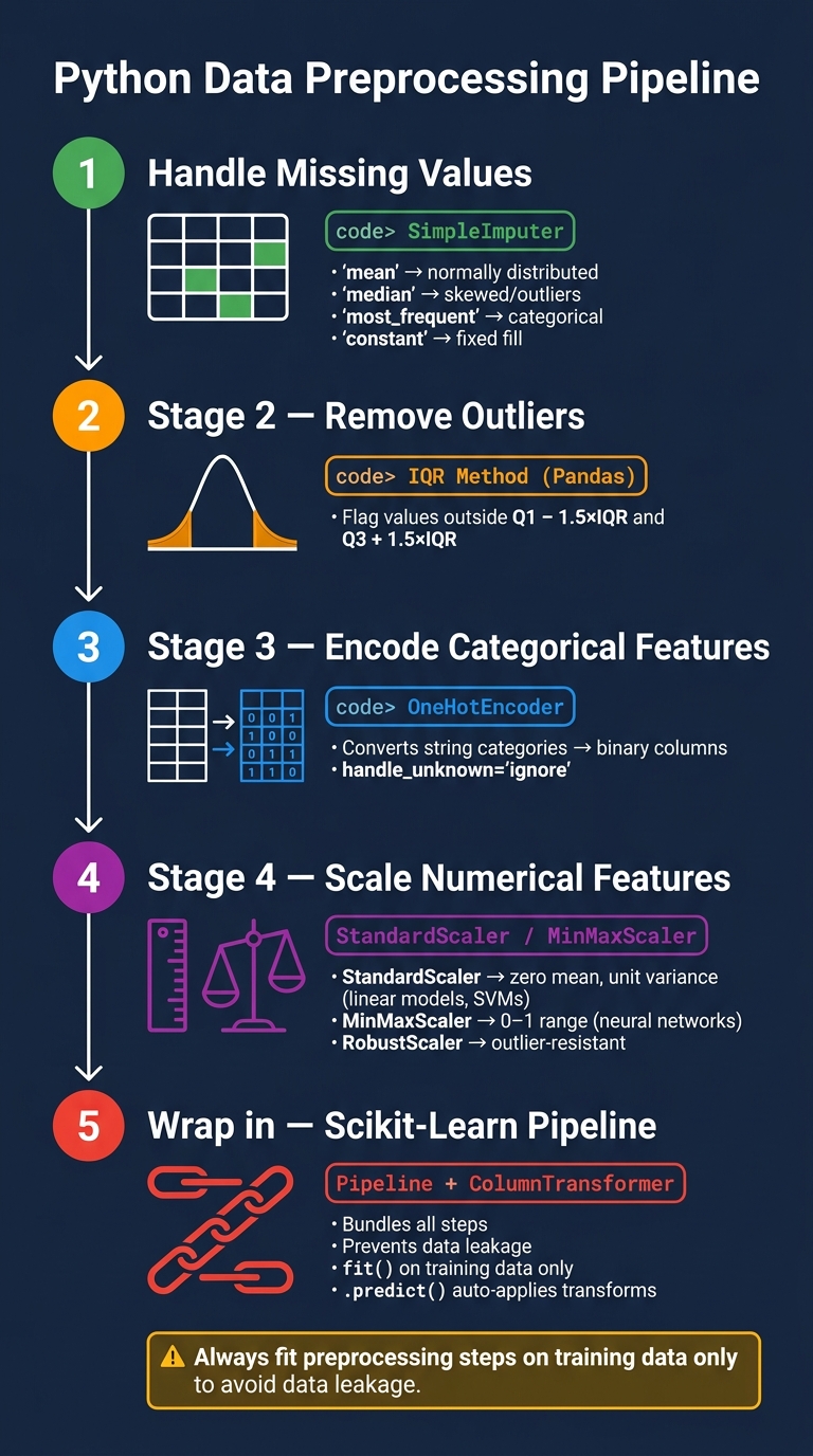
Python Data Preprocessing Pipeline: Step-by-Step Workflow
Manually running each transformation helps catch edge cases and understand their effects. Once these steps are validated, they can be automated into a pipeline.
Handling Missing Values with SimpleImputer
The SimpleImputer module in Scikit-Learn fills missing values based on statistics calculated for each column independently. The choice of strategy depends on the data type and distribution. For instance, the mean works well for normally distributed numerical data, while the median is better suited for skewed distributions or datasets with outliers. For categorical data, use most_frequent or constant. Attempting to apply numerical strategies like mean or median to string-based columns will result in errors.
from sklearn.impute import SimpleImputer
import numpy as np

imputer = SimpleImputer(strategy='median')
imputer.fit(X_train)
X_train_imputed = imputer.transform(X_train)
X_test_imputed = imputer.transform(X_test)
| Strategy | Data Type | Best Use Case |
|---|---|---|
| mean | Numeric | Normally distributed data without significant outliers |
| median | Numeric | Skewed distributions or data with outliers |
| most_frequent | Numeric or String | Categorical data or discrete numerical features |
| constant | Numeric or String | When missing values should map to a specific value |
Removing Outliers Using the IQR Method
Scikit-Learn does not include a built-in transformer for outlier removal, so this step is typically done with Pandas. The Interquartile Range (IQR) method identifies outliers by calculating the range of the middle 50% of values. Observations falling outside 1.5 times the IQR are flagged as outliers.
def remove_outliers_iqr(df, columns):
    mask = pd.Series([True] * len(df), index=df.index)
    for col in columns:
        Q1 = df[col].quantile(0.25)
        Q3 = df[col].quantile(0.75)
        IQR = Q3 - Q1
        lower = Q1 - 1.5 * IQR
        upper = Q3 + 1.5 * IQR
        mask &= df[col].between(lower, upper)
    return df[mask]

df_clean = remove_outliers_iqr(df, df.select_dtypes(include='number').columns)
For datasets like load_diabetes, only a small number of records may be removed, but this step becomes critical in noisier datasets.
After handling outliers, the next step is encoding categorical features.
Encoding Categorical Features with OneHotEncoder
For categorical data, OneHotEncoder converts each unique category into a binary column. This is particularly useful when dealing with string-based features.
from sklearn.preprocessing import OneHotEncoder
import pandas as pd

# Example with a synthetic categorical column
df['sex_category'] = df['sex'].apply(lambda x: 'male' if x > 0 else 'female')

encoder = OneHotEncoder(handle_unknown='ignore', sparse_output=False)
encoded = encoder.fit_transform(df[['sex_category']])
encoded_df = pd.DataFrame(encoded, columns=encoder.get_feature_names_out(['sex_category']))
Setting handle_unknown='ignore' prevents errors when the test set includes unseen categories. For linear models, consider drop='first' to avoid multicollinearity caused by redundant binary columns.
Scaling Features with MinMaxScaler and StandardScaler
According to Scikit-Learn's documentation, many machine learning algorithms require standardized input data to work effectively. StandardScaler standardizes features to have zero mean and unit variance, making it suitable for algorithms like linear models or support vector machines.
Alternatively, MinMaxScaler rescales features to a 0–1 range, which is especially helpful for neural networks. However, it is highly sensitive to outliers, so if outliers cannot be removed, RobustScaler may be a better option.
from sklearn.preprocessing import StandardScaler, MinMaxScaler

scaler = StandardScaler()
X_train_scaled = scaler.fit_transform(X_train_imputed)
X_test_scaled = scaler.transform(X_test_imputed)
By combining imputation, outlier removal, encoding, and scaling, you can create an efficient preprocessing pipeline in Scikit-Learn.
Note: Always fit preprocessing steps on the training set to avoid data leakage.
Automating Preprocessing with Scikit-Learn Pipelines
Running transformations one by one might work during exploration, but in production, it opens the door to data leakage. Scikit-Learn Pipelines address this by bundling all transformations into a single object that ensures everything happens in the right order. As of scikit-learn 1.8 (the 2026 stable release), pipelines also natively support pandas DataFrame outputs via set_output(transform="pandas").
Building a Pipeline for Numerical and Categorical Data
To handle both numerical and categorical data, you will need two tools working together. A Pipeline handles transformations for specific columns, while a ColumnTransformer directs subsets of columns to their respective pipelines and combines the results. You can even nest pipelines within the ColumnTransformer and wrap the entire setup in a final Pipeline that includes your estimator.
from sklearn.pipeline import Pipeline
from sklearn.compose import ColumnTransformer, make_column_selector as selector
from sklearn.impute import SimpleImputer
from sklearn.preprocessing import StandardScaler, OneHotEncoder

numerical_pipeline = Pipeline(steps=[
    ('imputer', SimpleImputer(strategy='median')),
    ('scaler', StandardScaler())
])

categorical_pipeline = Pipeline(steps=[
    ('imputer', SimpleImputer(strategy='most_frequent')),
    ('encoder', OneHotEncoder(handle_unknown='ignore', sparse_output=False))
])

preprocessor = ColumnTransformer(transformers=[
    ('num', numerical_pipeline, selector(dtype_include='number')),
    ('cat', categorical_pipeline, selector(dtype_include='object'))
],
remainder='passthrough')
Using make_column_selector keeps things flexible, automatically adapting to changes in the dataset's schema. The remainder='passthrough' setting ensures columns that do not need transformation are kept instead of being dropped without notice. That is a common pitfall. This design makes transitioning to model training straightforward.
Fitting and Transforming Data in One Step
With the ColumnTransformer defined, you can embed it into a final Pipeline that includes your model. By calling .fit() just once on the training data, you avoid data leakage. Each step in the pipeline applies fit_transform() internally, and the model trains on the fully transformed data.
from sklearn.linear_model import LogisticRegression

full_pipeline = Pipeline(steps=[
    ('preprocessor', preprocessor),
    ('model', LogisticRegression(max_iter=1000))
])

full_pipeline.fit(X_train, y_train)
print(f"Test accuracy: {full_pipeline.score(X_test, y_test):.3f}")
Once the pipeline is fitted, methods like .score() or .predict() automatically apply all transformations to new data before passing it to the model. You do not need to manually call .transform(). For debugging or understanding complex setups, you can configure your environment to display a diagram of the pipeline, which is particularly helpful for nested ColumnTransformer structures.
Comparing Data Distributions Before and After Preprocessing
The pipeline's fit_transform() method outputs a NumPy array by default, so you'll need a small conversion step for plotting (or call set_output(transform="pandas") on the preprocessor). To inspect how preprocessing changes your data, you can call preprocessor.fit_transform(X_train) separately before adding the estimator.
import matplotlib.pyplot as plt
import numpy as np

X_transformed = preprocessor.fit_transform(X_train)

fig, axes = plt.subplots(1, 2, figsize=(12, 4))
axes[0].hist(X_train.select_dtypes(include='number').iloc[:, 0], bins=30)
axes[0].set_title('Before: Raw Feature Distribution')
axes[1].hist(X_transformed[:, 0], bins=30)
axes[1].set_title('After: Scaled Feature Distribution')
plt.tight_layout()
plt.show()
After scaling with StandardScaler, you'll typically see values centered near zero, mostly within the range of –3 to 3. For categorical data, OneHotEncoder outputs binary columns. If a feature still has a strong skew after scaling, consider changing your imputation strategy or applying a log transform earlier in the pipeline.
Note: IfOneHotEncoderproduces a sparse matrix, setsparse_output=Falseor use.toarray()to convert it for plotting.
Once you are satisfied with the preprocessing results, the pipeline can be saved for reuse. Use joblib.dump(full_pipeline, 'pipeline.joblib') to save it and joblib.load() to reload it. This preserves all fitted parameters, like scaling factors and encoder mappings, exactly as they were during training.
Advanced Automation Options
Building on the foundational manual pipelines, advanced automation options can further simplify and standardize preprocessing tasks. These methods complement the reusability and clarity emphasized in earlier pipeline building while introducing tools to handle repetitive or complex steps more efficiently.
Writing Reusable Functions for Custom Preprocessing Tasks
While Scikit-Learn pipelines are powerful, they don't address a common issue: much of the data cleaning code is written inline, used once, and rarely revisited. Wrapping repetitive tasks into reusable components can alleviate this problem.
To create pipeline-compatible components, you can build a custom transformer class by inheriting from BaseEstimator and TransformerMixin. This approach involves defining a fit() method to calculate parameters from training data and a transform() method to apply those parameters. Here's an example of an OutlierClipper class that calculates interquartile range (IQR) bounds during the fit() stage and clips outliers during transform():
from sklearn.base import BaseEstimator, TransformerMixin
import numpy as np

class OutlierClipper(BaseEstimator, TransformerMixin):
    def fit(self, X, y=None):
        Q1 = np.percentile(X, 25, axis=0)
        Q3 = np.percentile(X, 75, axis=0)
        IQR = Q3 - Q1
        self.lower_ = Q1 - 1.5 * IQR
        self.upper_ = Q3 + 1.5 * IQR
        return self

    def transform(self, X):
        return np.clip(X, self.lower_, self.upper_)
This custom transformer can be seamlessly integrated into a Scikit-Learn pipeline. For simpler, stateless tasks (like applying log transformations or standardizing column names) FunctionTransformer is a convenient option. For example, you could use it to implement a clean_column_names function that converts column names to lowercase, strips whitespace, and replaces spaces with underscores.
Another useful feature in Scikit-Learn (version 1.2 and later) is set_output(transform="pandas"). This makes pipelines return pandas DataFrames instead of NumPy arrays, which helps preserve column names and simplifies debugging when inspecting intermediate outputs.
Using AutoClean for End-to-End Data Cleaning
If you're looking for a more automated approach, AutoClean offers a one-call solution for tasks like handling missing values, encoding categorical data, and detecting outliers. Its simple API is especially helpful for quickly preparing datasets during exploratory analysis. Here's an example:
from AutoClean import AutoClean

pipeline = AutoClean(df, mode='auto', missing_num='auto', encode_categ=['auto'])
clean_df = pipeline.output
AutoClean automatically identifies column types, selects imputation methods, and handles encoding with minimal configuration. While this makes it a fast option for creating a clean baseline, the tradeoff is reduced transparency. You may not have full visibility into the decisions made for each column, which could be a concern when explaining preprocessing choices or reproducing results.
For production environments, it is best to treat AutoClean as a starting point or diagnostic tool. Pair it with a schema validation tool like Pandera to ensure the output meets specific requirements and to catch potential issues that might be overlooked.
Manual Pipeline vs. AutoClean: Side-by-Side Comparison
Choosing between a manual Scikit-Learn pipeline and AutoClean depends on the stage of your project and the level of control you need. Here is how they compare:
| Feature | Manual Pipeline (Scikit-Learn) | AutoClean |
|---|---|---|
| Development effort | High. Requires writing custom functions and classes | Low. Minimal setup required |
| Customization | Full. Supports complex, domain-specific logic | Limited. Relies on predefined strategies |
| Production readiness | High. Easily serialized and fully testable | Moderate. Better for quick prototyping |
| Auditability | High. Every step is explicit and traceable | Lower. Internal processes are less visible |
| Data retention | Configurable. Can modify data without dropping rows | Varies. May drop or replace values by default |
For production workflows, manual pipelines offer more reliability, as they allow for explicit, testable, and traceable steps. AutoClean, on the other hand, shines during the exploratory phase, where speed and ease of use are more important than fine-grained control.
Checking Data Quality and Preparing for Modeling
These quality checks act as a safeguard for your automated pipeline, ensuring that the data it processes is ready for modeling. Even with automation, manual validation steps are crucial to catch potential issues.
Running a Correlation Check After Preprocessing
Use df.corr() to examine correlations among features and between features and the target variable. Look for near-zero correlations to identify irrelevant features and flag pairs with correlations above 0.9, as these may indicate multicollinearity, which can distort model performance.
Checking Class Balance in the Target Variable
Run y.value_counts() to inspect the distribution of classes in your target variable. For binary classification problems, a 90/10 split or more extreme imbalance can be problematic. Such skewed distributions may inflate accuracy metrics while ignoring poor performance on the minority class. If imbalance is detected, consider techniques like:
- Oversampling the minority class with SMOTE
- Undersampling the majority class
- Using
class_weight='balanced'in your model to adjust for class imbalance
"In machine learning, garbage in means garbage out. That's why automated data processing is not just a convenience, it's a necessity." - Khushi Bhadange
Splitting Data into Training and Test Sets
Divide your dataset into training and test sets using an 80/20 split. To ensure reproducibility, set a random_state, and if your target variable is imbalanced, use stratify=y to maintain the class proportions across splits:
from sklearn.model_selection import train_test_split

X_train, X_test, y_train, y_test = train_test_split(
    X, y, test_size=0.2, random_state=42, stratify=y
)
"We cannot use the same data for both training and testing... Otherwise, we would be causing data leakage, which basically means the model learning about the properties of the test data." - Soner Yıldırım
For projects involving hyperparameter tuning, reserve a validation set from X_train or use cross-validation techniques. Keep X_test untouched for the final evaluation. If you are handling time-series data, set shuffle=False during the split to preserve the chronological order.
FAQs
How do I avoid data leakage in preprocessing?
To avoid data leakage, always fit preprocessing steps like imputation or scaling exclusively on the training data. Once fitted, apply these transformations to the test data without re-fitting. Scikit-learn's Pipeline is a great tool for chaining these steps while maintaining this separation. When training, use the pipeline's fit() method with only the training data. For the test data, rely on predict() or transform() to apply the pre-fitted transformations, ensuring the model remains reliable and consistent.
When should I use StandardScaler vs MinMaxScaler?
When you need to standardize features by removing the mean and scaling to unit variance, StandardScaler is the go-to choice. This approach is particularly effective for algorithms that are sensitive to the scale of features, such as linear models and SVMs. However, it performs best when your dataset does not contain extreme outliers, as they can distort the scaling.
On the other hand, if you need to scale features to a specific range (say, between [0, 1]) MinMaxScaler is a better fit. This method is often used for algorithms that require bounded inputs, like neural networks. Keep in mind, though, that it is more vulnerable to outliers since the scaling factors are determined by the observed minimum and maximum values in the data.
How can I keep column names after a pipeline transform?
To keep column names intact after applying transformations in scikit-learn, you can use the verbose_feature_names_out=True parameter in transformers like ColumnTransformer. Alongside this, the set_output API is a useful tool for managing and retaining feature names. By configuring your pipeline with these options, you can ensure that the resulting DataFrame preserves the original column labels post-transformation.
Comments